Annotation Is the Bottleneck — Here’s How We Fixed It

Towards auto-annotation pipeline for object detection models

By Timotej Ponek
To train any computer vision model (CV) model for a specific task, you first need to have (relevant) data. The second thing is to annotate and curate this data. You need high-quality annotation, meaning precise bounding boxes and for individual samples to be varying, so your model is trained to generalize well to unseen data (data not present in training).
Gathering the data can take hours, and annotating takes days.

Standard workflow

At profiq we have experience with end-to-end CV model training for yolo and rf-detr architectures. The usual workflow when training a model was iterative, starting first with annotating some samples (a few dozen) by hand and then training the first “dummy” model to be used for the auto-annotation process.
Then we followed the iteration with these steps:

1. Use the model to auto-annotate more samples (or the remaining samples)
2. Go through the annotated samples and fix mistakes
3. Train the next model and go to point 1.

Bottleneck

As you can see, this workflow is iterative and the first iteration usually takes less than a day, but as the dataset grows, the iteration time grows with it.

Our approach

To speed up the annotation process we experimented with various approaches, like using Grounding DINO or roboflow’s autodistill framework, but the real breakthrough came with the release of SAM3. It added prompting by words, which was not present in SAM2 and is much more precise than in Grounding DINO. If your task is to detect cars or other general objects, you can use purely SAM3 without additional tools to create high-quality datasets. You will only need to tinker with the confidence threshold and implement a mechanism to filter overlapping annotations (which sometimes happens).
But if your task is to detect a special car model or brand, SAM3 might not be trained on that. In that case, you can use SAM3 to detect all cars, as the car is a general object. Afterwards, you will need to filter detections. You can do this all by hand, or iteratively train a classifier on a subset of the detections, classify the rest and fix mistakes. What are your options if you want to avoid the iterative training?

Similarity by embeddings

We experimented with using the embeddings generated by DINOv2 model of base size (768-dimensional embeddings per image). Why embeddings? In simple terms, embedding is a compact numerical representation that captures visual characteristics of the image. Instead of comparing images pixel by pixel, embeddings make it possible to compare them at a higher level, based on features such as shape, texture, and overall visual structure. As a result, images with similar content tend to have similar embeddings. Therefore, embeddings can be used in classification tasks.
Our idea was: What if we generate embeddings for all detections and for base images which represent our target class, calculate cosine similarity and classify those detections whose embeddings are similar to embeddings of base images as target class. Apart from cosine similarity, other approaches such as euclidean distance can be used, which might be better in some cases, but in our experiments those metrics were closely similar.

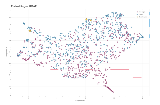
Caption 1: Embeddings for skoda dataset reduced by UMAP method into 2-dimensional space. You can see parts where target and non-target overlap, with some of the non-target samples forming a cluster in the bottom right (those are cutouts of trucks). Those samples will be distinguishable even with simple cosine similarity method.

Choosing threshold

With cosine similarities calculated, the next challenge was to determine at what point (threshold) a detection is considered similar enough to the target class to be labelled as such. The threshold can be selected manually by inspecting examples (for example in fiftyone), or calculated automatically if we label the detections. For that calculation we chose a strategy that maximizes F1 score, which aims to balance precision and recall.
However, at this point an important limitation was revealed. Many target samples were relatively similar to non-target samples. This is visible in the caption 1, where you can see that after reducing the embeddings to make them easier to inspect, the target class and non-target are heavily overlapping rather than forming clearly separated groups.
One approach to deal with this would be selecting specific parts of the embeddings that are most significant to us and giving them higher weight in the similarity computation. But since it is not easy to determine those parts, we came up with another idea to address our issue: What if we train embedding projector (MLP) that will project embeddings to lower dimensional space where target embeddings are closer to each other (or closer to base image embeddings) and non-target embeddings are further apart from target embeddings?

Embedding projector (MLP)

We trained a small multilayer perceptron (MLP) on top of the precomputed embeddings. Because MLP works only with embeddings rather than with full images, it is relatively lightweight and can be trained on consumer hardware.
We explored several training strategies, but the one that worked reliably was a contrastive approach. The idea is simple: in each epoch, pairwise distances between all sample pairs are computed and same-label pairs (both target vs target and non-target vs non-target) are pulled together while different-label pairs (target vs non-target) are pushed apart. In our case, this gradually reshaped the embedding space so that the dataset began to separate into the desired clusters after only a few training epochs.
For training, the annotated embeddings are split into training and validation sets. Base image embedding(s) is used to calculate validation accuracy, which is used to pick the best model and to decide whether to stop training if no improvement is observed for some number of epochs.

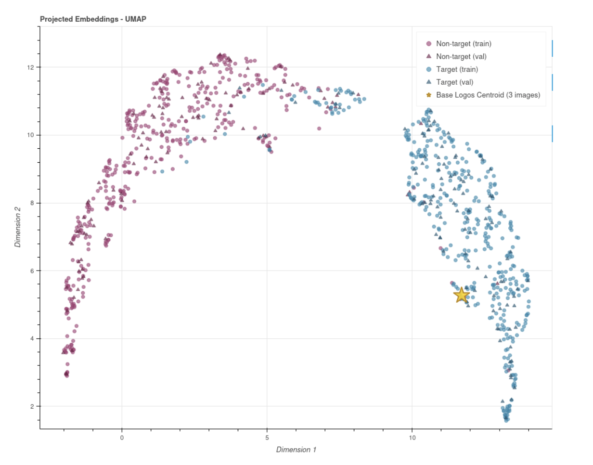
Caption 2: Embeddings for skoda dataset projected by the trained MLP with base image(s) centroid, reduced by UMAP method into 2-dimensional space. You can see a clear distinction between target and non-target, with some samples still overlapping.
Later, however, we found that this could be unstable: if the base images looked somewhat different from the real target samples in the dataset, they were not always a reliable guide for model selection. One straightforward improvement was to replace these external references with a centroid representation of the target class (calculated as the mean of non-projected target train split embeddings). The centroid provides a more stable and representative reference point for measuring how well the MLP clusters target embeddings, leading to better model selection.

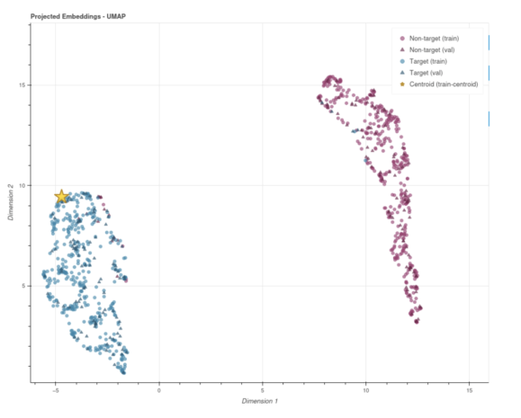
Caption 3: Embeddings for skoda dataset projected by the trained MLP with target train split centroid, reduced by UMAP method into 2-dimensional space. You can see that target and non-target samples are clearly apart from each other. Very few samples are still overlapping,

Extension to multiple classes

The advantage of MLP trained with contrastive metric is that it extends naturally beyond the binary case. The method does not depend on having only two classes; it simply uses label information to pull together samples that belong to the same class and push apart samples that do not. That means the same training approach can be reused for multi-class settings.

Comparison to training a classifier

Training a classifier instead of the MLP is also a valid option. There are few things to consider:

• Training speed: our MLP was trained in half or less time than comparable yolos/yolom classifier. We used the same patience (early stopping) parameter for both.

• Dataset size: here it is the same in both cases. More data = better model.

• Metrics: from our findings, both approaches give similar metrics. We see theoretically better generalization for MLP, as it is trained to “cluster embeddings”.

Our workflow for annotation

With the above said, in this section we will show how we used the described approach for creating a dataset to detect skoda cars. The images for the dataset were taken from traffic cameras in Brno city.

Dataset preparation for MLP training

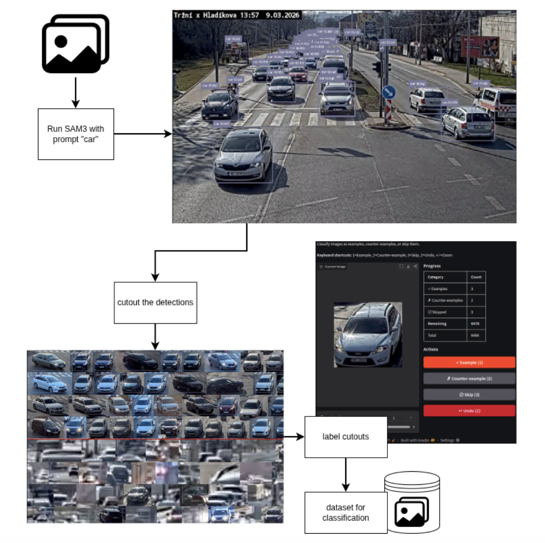
First we run SAM3 to detect all cars in the images. Then we extract the detections as separate images (only those with at least 2500 pixels, as on smaller cutouts you cannot see the difference between car brands). Next is the labelling. We care only about the front of the car, so all backs of the cars can be ignored/skipped or assigned to non-target class. We also skip cutouts that have no meaningful information (those where SAM3 detected a car with low confidence but looking at it we see only some blurry spots). After labelling we have a classification dataset that we can use to train MLP.

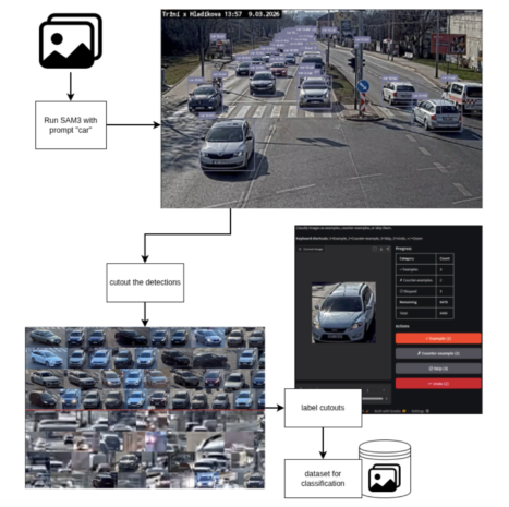
Caption 4: Diagram showing the flow of dataset preparation for training MLP. Same applies if you want to train a classifier instead.

MLP training

For MLP training, we first extract embeddings from our dataset and we are ready to train MLP. Afterwards, we can use MLP in an auto-annotation manner.

Autoannotation with MLP

The auto-annotation pipeline works in 3 phases:

• Phase 1 - use SAM3 to detect desired general object (“car”)
• Phase 2 - use DINOv2 to extract embeddings for SAM3 detections
• Phase 3 - use MLP to project embeddings and classify based on cosine similarity

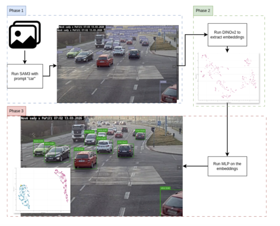
Caption 5: Diagram showing the use of MLP to annotate unseen data. If you trained a classifier, you replace Phase 2 & 3 with classification on cutouts.
On the image below you can see the output of auto-annotation pipeline (with class “other” hidden for clarity).

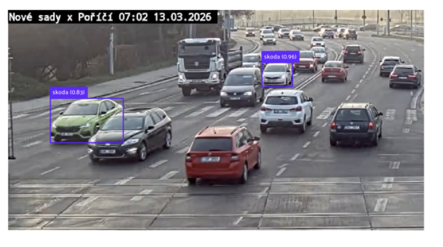
Caption 6: Annotated target class skoda (cosine similarity is above the threshold obtained from MLP training)

Closing thoughts

We did not explore auto-annotation tools provided by other platforms beyond roboflow. We also did not explore autolabelling options in local tools like LabelMe, AnyLabeling, X-AnyLabeling etc. If you have experience with other tools, feel free to share, we are interested in hearing how you do your annotations and your workflow.